Introduction

The airfoil is a critical component, particularly so in enabling flight. In essence, it is a curved surface that is designed to give the most favourable ratio of lift to drag. It has found application in a variety of domains, from aircraft and helicopters, to wind turbines. However, due to the complex behaviour of flow around an airfoil, noise-generation is a significant issue. Ablation of this selfgenerated noise is considered important for a few reasons: maintaining reasonable noise levels around wind farms allowing for human settlement; passenger comfort in aircraft and helicopters. This project attempts to develop a multi-variate regression procedure for the prediction of sound pressure levels (SPL) of the generated noise, utilizing data collected via extensive acoustic and aerodynamic wind tunnel testing. SPL is simply a representation of the intensity of the sound pressure wave generated from the airfoil, measured at a standardized distance. Figure 1 details the location of the airfoil on an aircraft and defines some basic nomenclature.

Noise prediction, particularly from a complex flow phenomena such as flow over an airfoil is a challenging task - requiring the implementation of extensive experimental, analytical and numerical techniques to ensure a reliable prediction. Rather than attempting to predict noise with the regression analysis, the motivation behind this work is to examine the effect of various explanatory variables on the SPL, and explore how well such an analysis fits the experimental data. Also, various techniques of model building, diagnostics and remedial measures were performed on the data.

Description of the data set

The data set represents a collection of extensive experimental data obtained via wind tunnel testing. The data set was acquired from the UCI machine learning repository[1]. The response variable is represented as Yˆ and the explanatory variables are represented as Xi.

Yˆ - Sound Pressure Level (SPL) in decibels (dB)

X1 - Frequency in Hertz (in Hz)

X2 - Angle of attack (in degrees)

X3 - Chord length (in metres)

X4 - Free stream velocity (in metres per second)

X5 - Suction side displacement thickness (in metres)

It is to be noted that the frequency refers to the frequency at which the SPL is measured. Also, the suction side displacement thickness refers to the boundary layer thickness of the air over the airfoil measured at a defined distance from the airfoil surface[2]. Figure 2 shows some more nomenclature pertaining to the explanatory variables.

Procedure

The multivariate regression procedure was applied to analyze the experimental data. SAS was extensively utilized at all stages of the project, and the code utilized for the project has been attached in the appendix. Most of the concepts explained in the below paragraphs are comprehensively explained in our reference text[3].

Exploratory data analysis

The scatter plot matrix generated by SAS was employed to study the relationship between the explanatory variables. This simple tool gives us a qualitative idea of the variables and helps us identify any possible sources of multi-collinearity. Figure 3 shows the scatter plot matrix, and it is immediately evident that there is some positive relationship between the angle of attack and the suction side displacement thickness. From the standpoint of physics, this is not very surprising - an increase in the angle of attack results in a stronger adverse pressure gradient generated over the suction (top) side of the airfoil. The normal pressure gradient drives the fluid from the leading edge to the trailing edge of the airfoil[2]. Conversely, the adverse pressure gradient hampers this gradient and this results in fluid residing in the boundary layer to be pushed off the surface of the airfoil. Intuitively, this should result in an increase in the boundary layer thickness, as seen in the statistical data.

This effect will be quantified when we study multi-collinearity and we will use certain diagnostic tools to potentially remove one of the explanatory variables.

Model selection

Before fitting an equation, it is necessary to determine if all of the given explanatory variables are required in the model, or will a subset of the variables suffice. We use two popular procedures to assist in answering this question, namely the Mallow’s Cp criterion and the stepwise selection procedure.

Mallow’s Cp criterion

This criterion compares various subset models with the full model, and helps in eliminating bias in the predicted values. A model is considered good if it satisfies -

Cp ≤ p

In our case, p = 6. Table 1 clearly shows that only the full model with all explanatory variables included satisfies the test.

Stepwise selection procedure

This procedure adds explanatory variables one at a time using the general linear test; while looking back at every step to see if any variable can be removed. For the number of explanatory varibales in our model, this test is expected to perform reasonably well. As seen in Table 2, this procedure again suggests a model with all the explanatory variables included.

Based on the two tests detailed, we conclude that all explanatory variables need to be included in the model.

Multivariate linear regression

SAS was utilized to fit a regression equation to the experimental data. Table 3 details the ANOVA table for the regression, with the estimates for the parameters of the explanatory variables and 95% confidence intervals.

Yˆ = 132.83381 − 0.00128X1 − 0.42191X2 − 35.68800X3 + 0.09985X4 − 147.3005X5

The R2 value for the analysis is 0.5157, and the adjusted R2 value is 0.5141, implying little penalty due to the predictor variables. It can be seen that the marginal F test produces a very low pvalue (< 0.0001) allowing us to reject the hypothesis that all the regression coefficients are zero. Individual t-tests for the regression coefficients all produce extremely low values, allowing us to conclude that with the other coefficients included in the model, each regression coefficient is not zero.

Model diagnostics

The assumptions we check during model diagnostics are: whether the data violates the normality assumption; whether the residuals violate the constant variance assumption; whether there are severe outliers in the residuals.

Assumption of normality

Construction of a histogram and qq plot (Figure 4 and Figure 5) suggests that apart from at extreme values, the assumption of normalcy of the predicted SPL does not seem significantly violated. The histogram suggests some left-skewness in the data while the qqplot shows deviation from normal behaviour at the higher quantiles.

Assumption of constant variance

To check the assumption of constant variance, the residuals are plotted against the explanatory variables and the predicted values (Figure 6). We can immediately notice that there is evidence of non-constant variance in the plots of frequency, chord length and suction side displacement.

Multi-collinearity

As mentioned earlier, the potential multi-collinearity between the angle of attack and the suction side displacement is investigated in this section.

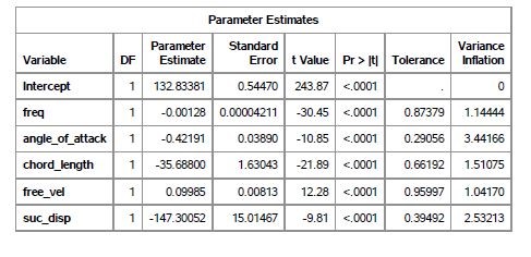
First, as a qualitative measure the difference in SS1 and SS2 errors were seen in Table 3. The lack of significant difference indicates that severe multi-collinearity is unlikely. Next, we construct the Pearson’s correlation coefficients matrix (Table 4) . We can see the two explanatory variables have a correlation coefficient of 0.75339. This value, while not low, was deemed not an indicator of severe multi-collinearity. To confirm this decision, we also utilize the Variance Inflation Factor (VIF) analysis. To rule out any possiblity of multi-collinearity, the VIF for each explanatory variable should be -

VIFi > 10

Table 5 confirms that the VIF value does not exceed 10 for any explanatory variable, and we can conclude that there are no severe multi-collinearity issues in our model.

Identifying outliers

To identify data points that can be classified as outliers, we use studentized deleted residuals as a measure. For a value to be considered an outlier, the absolute value of the residual should be greater than the critical value 4.1625, as determined from the inverse t test. Figure 7a shows the residuals plotted against the SPL, confirming that there are no outliers in the data.

Influential observations

We use three measures to identify observations that are influential to the fitted regression line. This implies that when these observations are deleted, the fitted regression equation changes substantially. First, to measure the influence of observations with respect to the predicted value, we use the DFFITS parameter; the critical value for which is 0.12636. Figure 8 shows a few observations that are judged to be influential to the regression.

The leverage is used to determine if the predicted value is influential by virtue of how far the predictor values for this case is from the center of all predictor variables. The critical value for this parameter is determined to be 0.00798. Figure 7b shows a few observations beyond the critical value, marking them influential.

Finally, the DFBETAS parameter measures the influence of a particular case on each of the regression coefficeints. The critical value for this parameter is determined to be 0.05158. The plot for each regression coefficient is shown in Figure 9, and it is observed that a handful of observations are deemed influential (particularly for frequency).

Remedial measure

The non-constant variance with respect to some of the explanatory variables has already been discussed earlier in the report. The weighted regression technique was explored as a potential remedial measure for this issue. This technique applies a weight to each of the squared residuals, proportional to the inverse of the variance of the residual. SAS was utilized to implement this procedure and the results have been summarized in Figure 10.

The results show a small change in variance of residuals, particularly with respect to frequency and suction side displacement thickness. However, the remedial measure was not deemed to be very effective in improving the constancy of the residuals.

Summary of analysis

In summary, first some exploratory data analysis was performed with a scatter plot matrix to visually identify multi-collinearity issues. Model selection was then performed using the Mallow’s Cp criterion and the stepwise selection procedure. After verifying the necessity of using all explanatory variables, the regression equation was computed and a few conclusions were made using the f-test and t-tests for the variables.

Model diagnosis was then performed, wherein the assumptions of normality and constant variance was checked and issues were highlighted. The issue of potential multi-collinearity was explored, and it was satisfactorily concluded that there is no severe issue of multi-collinearity. The model was then checked for outliers and influential observations were highlighted.

Finally, a remedial measure was implemented, but was found to be not very effective.

Conclusion

In conclusion, despite a low R2 value obtained for the analysis, it can be said that the SPL of generated noise undeniably depends on the frequency, angle of attack, chord length, free stream velocity and the suction side displacement thickness.

Apart from developing a regression equation, some model diagnosis was performed and apart from checking of model assumption; aspects such as multi-collinearity, outliers and influential observations were explored. Fianlly, a remedial measure was suggested for the non-constant variance observed during model diagnosis.

References

1. Lichman M., UCI Machine Learning Repository, [http://archive.ics.uci.edu/ml], Irvine, CA: University of California, School of Information and Computer Science.

2. Brooks T.F., Pope D.S., Marcolini A.M., Airfoil self-noise and prediction; Technical report; NASA RP-1218; July 1989.

3. Kutner M.H., Neter J., Nachtsheim J., Li W., Applied linear statistical models, Irwin/McGraw Hill 2004.

Appendix

Figures

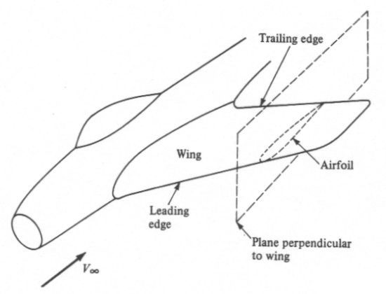
Figure 1: Basic features of an airfoil

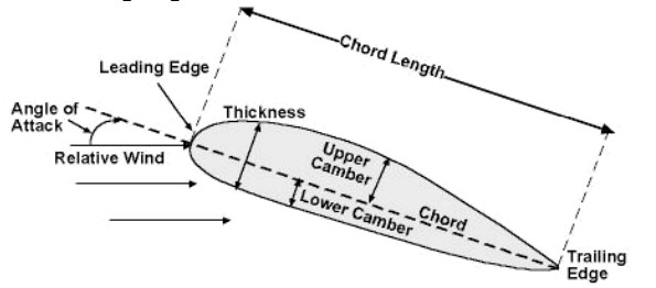
Figure 2: Detailed view of an airfoil with nomenclature

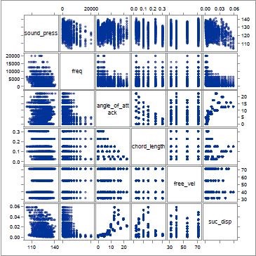
Figure 3: Scatter plot matrix

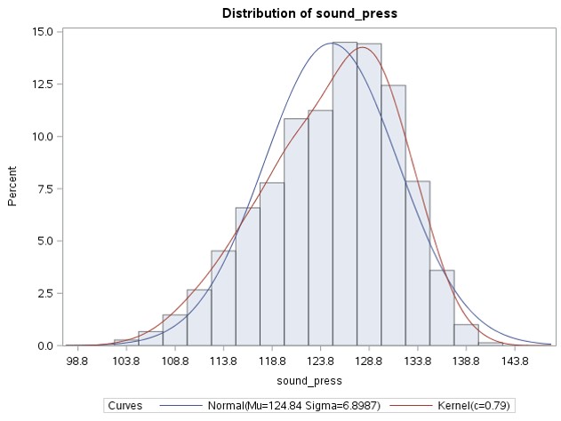
Figure 4: Histogram of SPL

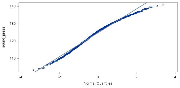
Figure 5: qq plot of the SPL with respect to the normal quantiles

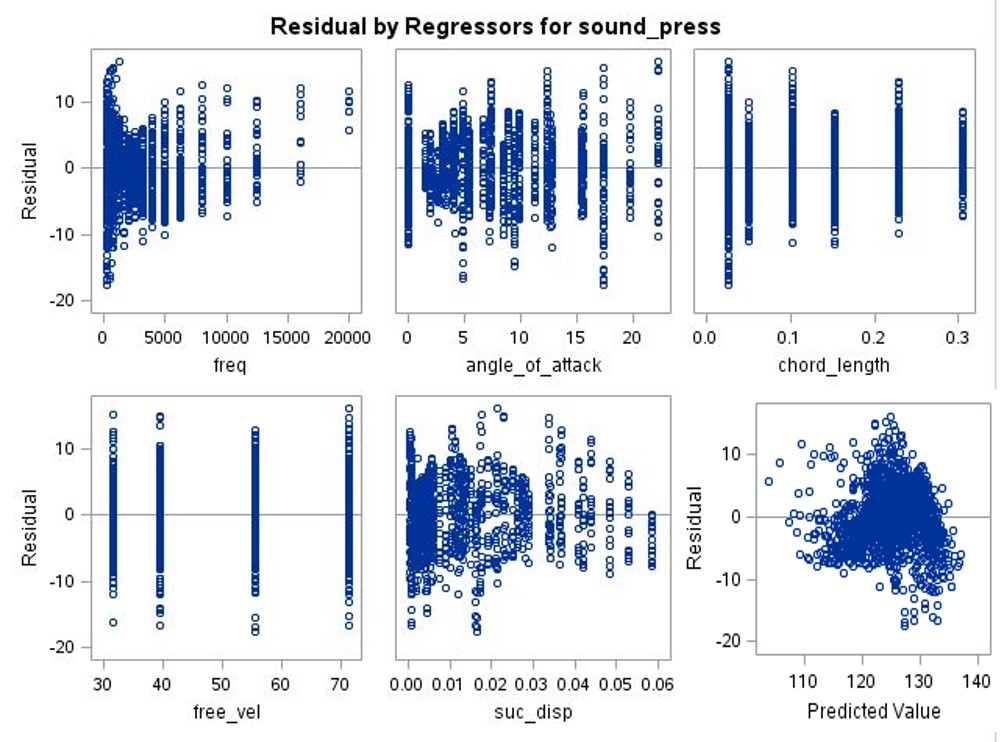
Figure 6: Residuals vs. explanatory variables and predicted variable

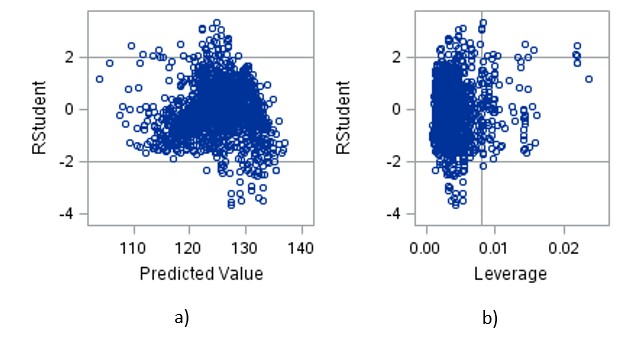
Figure 7: a) Deleted studentized residuals vs. predicted variable; b) deleted studentized residuals vs. leverage

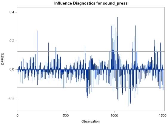
Figure 8: a) DFFITS plotted against the observation number

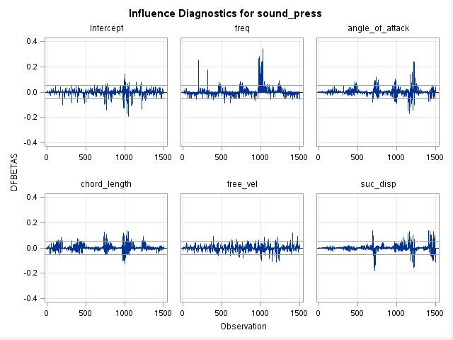
Figure 9: a) DFBETAS plotted against the observation number for each regression coefficient

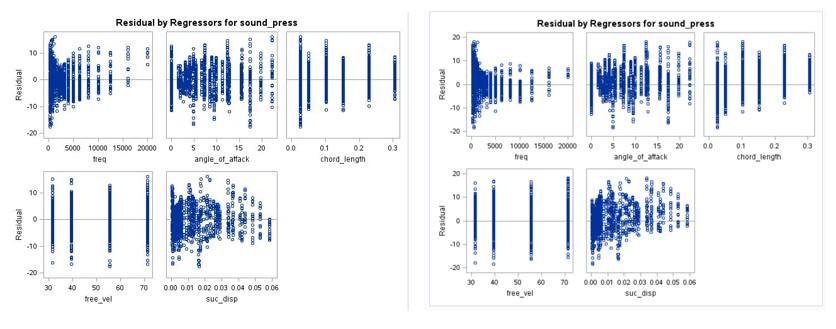
Figure 10: Comparison of residuals vs. explanatory variables before and after remedial measure

Tables

Table 1: Table showing the Mallow’s Cp values

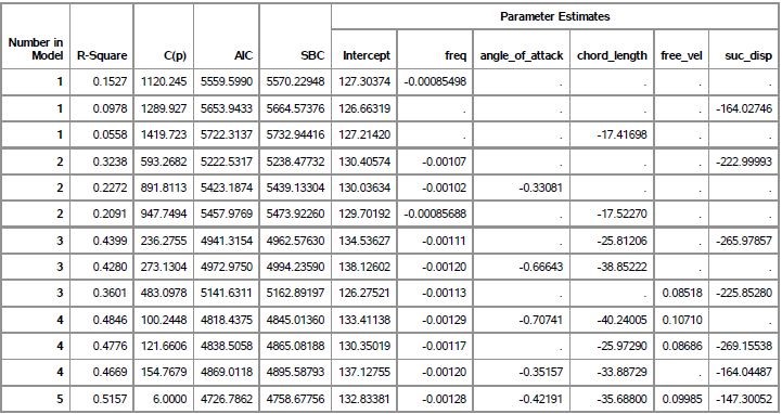
Table 2: Illustration of stepwise selection procedure

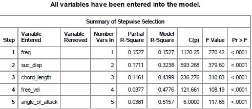
Table 3: ANOVA table for the multivariate regression

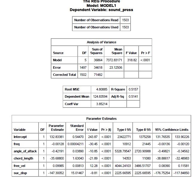
Table 4: Pearson’s correlation coefficients to assess multi-collinearity

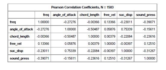
Table 5: Variance Inflation Factor analysis

Code used for the project

data airfoil ;

infile "/home/bhatnasa0/sasuser.v94/Airfoil_data1.csv" firstobs =2 dlm= " , " ;

input freq angle_of_attack chord_length free_vel suc_disp sound_press

\@\@;

run ;

proc print data= airfoil;

\*model selection ;

proc reg data= airfoil;

model sound_press=freq angle_of_attack chord_length free_vel suc_disp

/selection= adjrsq cp aic sbc best =3 b ;

run ;

\*stepwise selection;

proc reg data= airfoil;

model sound_press= freq angle_of_attack chord_length free_vel suc_disp

/ selection

run ;

\*regression;

proc reg data= airfoil;

model sound_press=f r eq angl e \_of \_ a t t a ck chord_length f r e e \_ v e l
suc_disp/ clm c lb output out=sound_press p=pred r=r e s id ;

\_proc univa r i a t e data= a i r f o i l plot ;

\_var r e s id ;

\_ checking mu l t i c o l l i n e a r i t y ;

proc s g s c a t t e r data= a i r f o i l ;

matrix sound_press f r eq angl e \_of \_ a t t a ck chord_length f r e e \_ v e
l suc_disp

;

run ;

\_ c o r r e l a t i o n matrix ;

proc cor r data= a i r f o i l noprob ;

\_ di agnos t i c ;

13

proc reg data= a i r f o i l ;

model sound_press=f r eq angl e \_of \_ a t t a ck chord_length f r e e \_ v e l
suc_disp/r inf luenc proc reg data= a i r f o i l ;

model sound_press=f r eq angl e \_of \_ a t t a ck chord_length f r e e \_ v e l
suc_disp/v i f t o l ;

\_ p a r t i a l plot ;

proc reg data= a i r f o i l ;

model sound_press=f r eq angl e \_of \_ a t t a ck chord_length f r e e \_ v e l
suc_disp/r p a r t i a l \_graph for di agnos t i c ;

ods graphi c s on ;

proc reg data= a i r f o i l

plot s =(CooksD RStudentByLeverage DFFITS DFBETAS ) ;

model sound_press=f r eq angl e \_of \_ a t t a ck chord_length f r e e \_ v e l
suc_disp ;

run ;

ods graphi cs o f f ;

\_ remedial ;

proc reg data= a i r f o i l ;

model sound_press=f r eq angl e \_of \_ a t t a ck chord_length f r e e \_ v e l
suc_disp ;

weight f r eq angl e \_of \_ a t t a ck chord_length f r e e \_ v e l suc_disp ;