Multivariate Analysis
OBJECTIVE- The data I’m studying here is biting fly data. There are 70 observations on two species of biting flies with 7 variables as:
X1 = wing length
X2 = wing width
X3 = third palp length
X4 = third palp width
X5 = fourth palp length
X6 = length of antennal segment 12
X7 = length of antennal segment 13
-
Perform a principal component analysis.
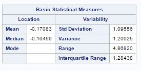
The principal component analysis helps in reducing the size of the variables. The principal components are the linear combinations of the random variables in data. Before principal component analysis, let’s look at the summary of our variables in fig-1:
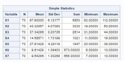
Fig-1
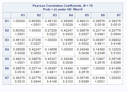
Fig-2
If we look at the correlation matrix of the variables in fig-2, we can see that variables are correlated with each other. So, we can move further in principal component analysis.
For this principal component analysis, principal component are calculated from the variance-covariance matrix of variables in fig-3.
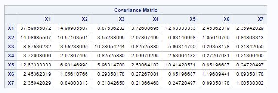
Fig-3
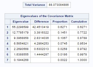
Fig-4
From fig-4, we can see that the sum of the eigen values is equal to the total variance. Also the eigen values are the variance of the principal components. The column proportion tells about the proportion of total population variance explained by the principal component. We can see that two components accounts for 77 percent of the total variance.
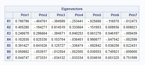
Fig-5
Since principal components are the linear combination of variables. They are of the form:
, i=1,2,..7 Here e is the eigen vector.
The magnitude of eik shows the importance of the kth variable to the i-th principal component, irrespective of the other variables. So fig-5 shows the importance of different variables(X1,X2,..X7) in the principal components. The one thing which we can notice that X1 has highest coefficient (0.781) in the principal component-1. This means that X1 has the highest weightage in principal component-1.Also coefficients for other variables are also positive but in decreasing order. For principal component-2, the variables X3, X4 and X5 have positive coefficients and other variables have negative coefficients, this seems that principal component is representing palp length over other features of biting fly.
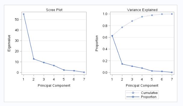
Fig-6
The scree plot in figure-6 helps in finding out the appropriate number of principal components. If we look at the scree plot, the elbow (bend) is at
- So if we choose two principal components then they are representing only 77% of the total variance from fig-4. There is also bend at 5 after position 2 and 4 principal components are account for 95% of the total population variance (fig-4). So I choose 4 principal components instead of 5. Because after 4, subsequent components contribute less than 2percent each (fig-4).
From fig-7, we can see the summary statistics of the seven principal component. The correlation matrix shows that principal components have 0 covariance and they are independent.
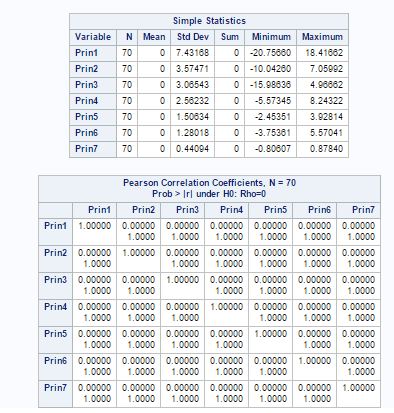
Fig-7
If I do choose first two principal components which account for 77% of the total population variance (fig-4). I can plot the two components with species. From the plot in fig-8, we can see that species (“1”) has higher values for all the variables than species (“0”). From the plot, we can see that for both species principal component2 value is on the higher side.
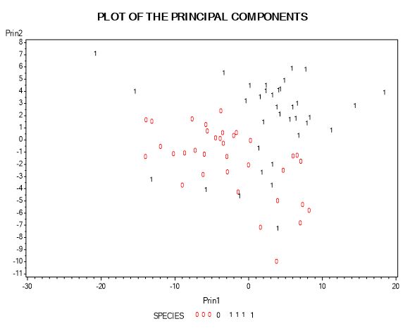
Fig-8
-
Perform a factor analysis. Interpret factors.
The factor analysis also helps in data reduction by reducing the number of observed variables with little loss in information. The highly correlated variables are grouped to form a factor and they have small correlation within different groups.
To find the appropriate number of factors, the method of principal component is applied. From fig-9 we can see that first two factors are the major one accounting for 63% of the total population variance. The proc factor procedure in sas also choose two factors. This can be clearer from the scree plot in fig-10. There is a sharp bend at 2.
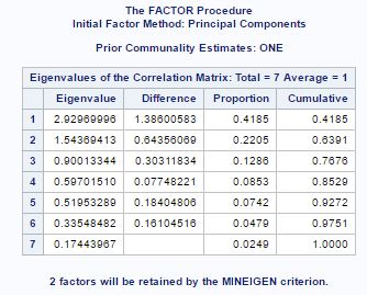
Fig-9
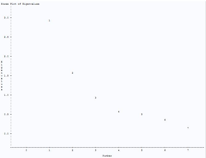
Fig-10
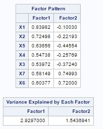
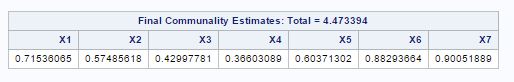
Fig-11
From fig-11, factor pattern shows that variable X1 has the highest positive value for factor-1 and X3 has lowest but X4, X3 and X7 have almost same values. For factor-2 X6 and X7 have the largest positive values.
From fig-12, we can see that factor X1, X2, X3, X4and X5 are closer to the positive side of fator1 and variables X6 and X7 are in between factor-1 and factor-2. Also variables X1, X2, X3, X4 and X5 are on the negative side of fator-2 and X6 and X7 are on the positive side of factor-2
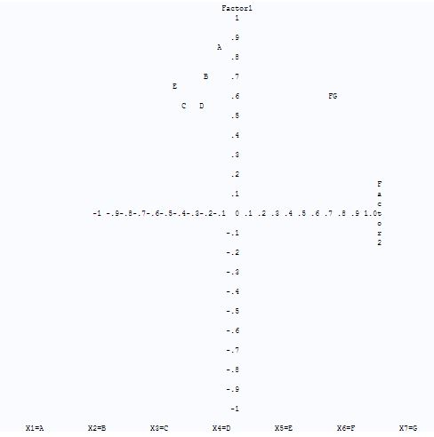
Fig-12
Since separation is not clear within variables for factor-1 and factor-2, hence I applied rotation.
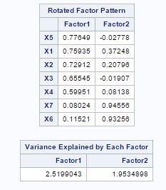
Fig-13
From fig-13, after rotation by varimax method, we can see that for factor-1, variables X5 has highest value now and variables X5,X1,X2,X3,X4 form a group for factor-1 with correlation>0.5 and for factor-2, variables X7 and X6 are forming a group. From fig-14, now we can clearly see two groups. One group or cluster of variables X1, X2,X3,X4 and X5 which is closer to factor-1 and other group of variables X6 and X7 which is closer to factor-2. Also variables X3 and X5 are lie along the axis of factor-1 with variable X4 lying very close to axis of factor-1. Variable X1 and X2 lying on the positive side of factor-2 but closer to positive side of factor-1. And variables X6and X7 are lying in the positive side of factor-2.
So the factor-1 which has X1,X2,X3,X4 and X5 variables reflects the wing and palp dimensions of the biting fly and factor-2 which has X6 and X7 variables reflect the properties of antenna of biting fly.
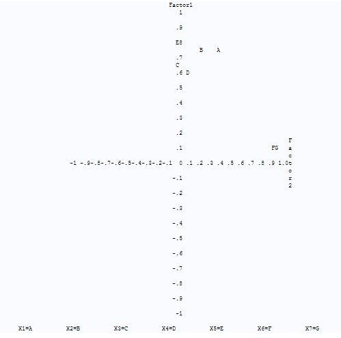
Fig-14
-
Plot the data……… Label species… Comment on plots…… Unusual points???
In the fig-15, the two species are plotted against two factors. From the plot, we can see that the highlighted point from species (“0”) can be a potential outlier. The values for species (“1”) are more spread out. Wing dimensions and palp dimensions for species (“1”) are higher than species (“0”). The length of antennal segments for both species are comparable. There is no clear classification of some observations for two species.
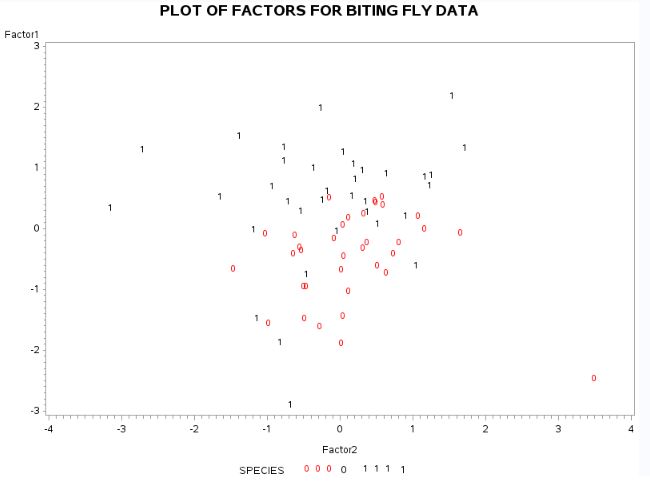
Fig-15
d) What seems to be the characteristics of the species with respect to the variables/factors??
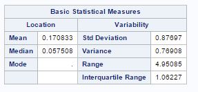
The characteristics of species with respect to variables are given by seven variables as wing length(X1), wing width(X2), third palp length(X3), third palp width(X4), fourth palp length (X5), length at antennal segment 12 (X6)and length at antennal segment 13.(X7). But after factor analysis, now we have two main factor, factor-1(X1, X2, X3, X4, X5) with wing and palp dimensions and factor-2 (X6, X7) with length of antennal segments. The summary of factors for different species is given as
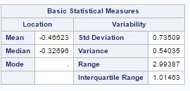
Factor-1 species (“0”) Factor-2 species (“0”)
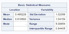
Factor-1 species (“1”) Factor-2 species (“1”)
The mean and variance for factor-1 is low for species(“0”) as compared to species(“1”) and mean for factor-2 is lower fore species(“1”) as compared to species(“0”).
e) Perform a discriminant analysis
The goal of discriminant analysis is to distinguish between different features of observations from different populations. The discriminant analysis starts with the assumption of equal variance between different populations. And there are different ways to do discriminant analysis when variances of populations are same or not.
Fig-16 shows the summary of data by showing total number of variables and class variables. The prior probabilities are assume to 0.5 each for both species.
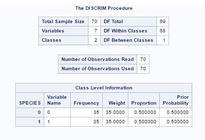
Fig- 16.
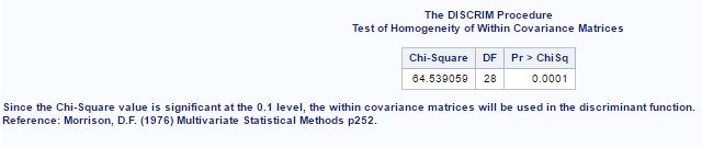
Fig-17
Fig-17 shows the test for equal variance. The null hypothesis tested here that variance between populations is same. Since p-value<0.05, at significance level of 0.05, null hypothesis of equal variances is rejected and quadratic classification rule is used as shown in fig-18.
From fig-18, we can see that 97.14% observation of species (“0”) correctly classified as species (“0“) and 91.43%observation of species (“1”) correctly classified as species (“1”). And error count is very low.
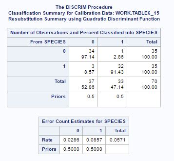
Fig-18
Since here we have 7 variables to start from, the other way is to first select variables from stepwise selection procedure. Fig-19 shows the summary of the stepwise procedure:
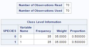
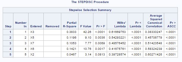
Fig-19
At significance level of 0.15, variables X2, X3, X5, X6 and X7 are selected. So now the discriminant analysis will be applied on these 5 selected variables.
Fig-20 shows the initial information about data, now instead of 7 variables before, now we have just 5 variables. The prior probability for both species is 0.5.
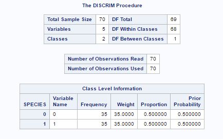
Fig-20
The test for equal variance for both species gave the result that variance for both species is different (fig-21).
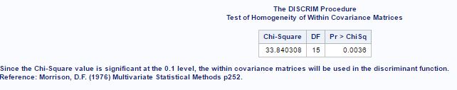
Fig-21
Hence the Quadratic classification rule has applied.
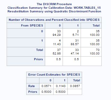
Fig-22
Fig-22 shows that 94.29% observation of species(“0”) are correctly classified as species(“0”) as compared to 97.14%(fig-18) and only 88.57% observation of species(“1”) are correctly classified as species(“1”) as compared to 91.43%(fig-18). And rate of error has also increased compared to the previous analysis when we had 7 variables. This may be because we have reduced the number of variables and so lost a little bit of information from data.
f) Perform a Multivariate analysis of variance on species w/r to variables and factors.
First the MANOVA analysis is on the actual variables of the data
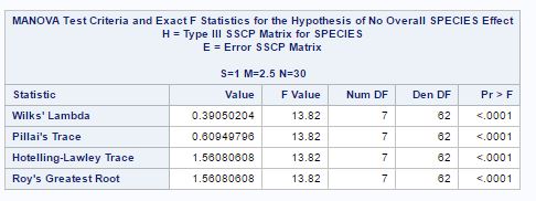
Fig-22
The model we have used here:
(1)
where j=1, 2,..nl (number of observation under each species), l=1,2 for species (1)
The null hypothesis is that mean for two species is same. The sas output in fig-22 gives so many statistics to test the null hypothesis. From the Wilk’s lambda statistic we can see that p-value is too small, so we reject null hypothesis and conclude that there is a significant difference in mean for species (“0”) and (“1”). If we look at other species as well, the p-value is small.
MANOVA for factor analysis.
From the factor analysis in problem-(b), we got two factors, so we can apply MANOVA on factor variables using factor scores.
Again we are using the same model (1) and same hypothesis as I have used before but instead of seven variables now I have two variables (factors).
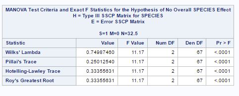
Fig-23
Here from fig-23, we can see that p-value is very low<0.0001 and hence we reject null hypothesis of equal means for two species and conclude that the mean for two species is different. The other statistics also giving the same conclusion.
Note: - 1.The one thing which is important here that the assumption of constant variance is violated here as we have tested before in fig-17. The one of the assumption of MANOVA is population (here two species) have equal variance but here we have tested that species “0” and “1” have different variance.
-
Also I have assumed here that both species are multivariate normally distributed.
-
And species (“0”) is independent from species (“1”).
APPENDIX
SAS CODE
   \* Data ;

   \*X1 = wing length

   X2 = wing width

   X3 = third palp length

   X4 = third palp width

   X5 = fourth palp length

   X6 = length of antennal segment 12

   X7 = length of antennal segment 13;

   DATA TABLE6_15;

   INPUT X1 X2 X3 X4 X5 X6 X7 SPECIES \@\@;

   CARDS;

   85 41 31 13 25 9 8 0

   87 38 32 14 22 13 13 0

   94 44 36 15 27 8 9 0

   92 43 32 17 28 9 9 0

   96 43 35 14 26 10 10 0

   91 44 36 12 24 9 9 0

   90 42 36 16 26 9 9 0

   .

   .

   .

   99 45 42 15 32 10 9 1

   102 45 44 15 30 10 10 1

   97 45 37 15 32 10 9 1

   96 39 40 14 20 9 9 1

   89 39 33 12 20 9 8 1

   99 42 38 14 33 9 9 1

   110 45 41 17 36 9 10 1

   99 44 35 16 31 10 10 1

   103 43 38 14 32 10 10 1

   95 46 36 15 31 8 8 1

   101 47 38 14 37 11 11 1

   103 47 40 15 32 11 11 1

   99 43 37 14 23 11 10 1

   105 50 40 16 33 12 11 1

   99 47 39 14 34 7 7 1

   ;

   proc print data=TABLE6_15;

   \* Principal Component Analysis;

   proc corr data=TABLE6_15;

   var X1 X2 X3 X4 X5 X6 X7;

   proc princomp data=TABLE6_15 cov out=aa outstat=aa_stat;

   var X1 X2 X3 X4 X5 X6 X7;

   run;

   proc score data=TABLE6_15 score=aa_stat out=FScore;

   var X1 X2 X3 X4 X5 X6 X7;run;

   GOPTIONS RESET=ALL;

   proc corr data=aa; \*the principal components are uncorrelated/independent;

   var prin1-prin7;

   run;

   proc gplot;

   title 'PLOT OF THE PRINCIPAL COMPONENTS';

   plot prin2\*prin1=species;

   symbol1 v=0 c=red;

   symbol2 v=1 c=black;

   run;

   \*quit;

   \* Factor Analysis;

   proc factor res rotate=v reorder plot scree;

   var X1 X2 X3 X4 X5 X6 X7 ;

   run;

   proc factor res rotate=v reorder n=2 out=ff out_stat=ff_1 plot scree;

   var X1 X2 X3 X4 X5 X6 X7;

   run;

   proc score data=TABLE6_15 score=ff_1 out=FScore;

   var X1 X2 X3 X4 X5 X6 X7; run;

   proc print data=FScore;run;

   proc corr data=ff;

   run;

   proc gplot;

   title 'PLOT OF FACTORS FOR BITING FLY DATA';

   plot factor1\*factor2=species;

   symbol1 v=0 c=red;

   symbol2 v=1 c=black;

   run;

   quit;

   \* MANOVA with factor analysis;

   PROC GLM DATA=FScore;

   CLASS SPECIES;

   MODEL factor1 factor2=SPECIES/ss3;

   MANOVA H=SPECIES;

   RUN;

   \* summary of factors;

   PROC UNIVARIATE data=FScore;

   VAR factor1 factor2;

   BY species;

   OUTPUT min=min mean=mean q1=q1 median=med q3=q3 max = max out=stats;

   RUN;

   \* Discriminant Analysis;

   \*with pool test;

   proc discrim data= TABLE6_15 pool=test wcov short ;

   \*this will test the equality of the variance covariance matrices;

   class species;

   var X1 X2 X3 X4 X5 X6 X7 ;

   run;

   \*with pool test=yes;

   proc discrim data= TABLE6_15 pool=yes out=out outd=outd;

   \*we will pool in this example if though it is inappropriate;

   class species;

   var X1 X2 X3 X4 X5 X6 X7 ;

   run;

   proc print data=out;

   proc print data=outd;

   \*stepwise discriminant analysis;

   proc stepdisc data=TABLE6_15;

   class species;

   var X1 X2 X3 X4 X5 X6 X7 ;

   run;

   \*proc discrim data= TABLE6_15 pool=test wcov short;

   \*this will test the equality of the variance covariance matrices;

   \*class species;

   \*var X2 X3 X5 X6 X7 ;

   run;

   \* MANOVA;

   PROC GLM DATA=TABLE6_15;

   CLASS SPECIES;

   MODEL X1 X2 X3 X4 X5 X6 X7=SPECIES/ss3;

   MANOVA H=SPECIES;

   RUN;